Shapley value, SHAP, Tree SHAP 설명

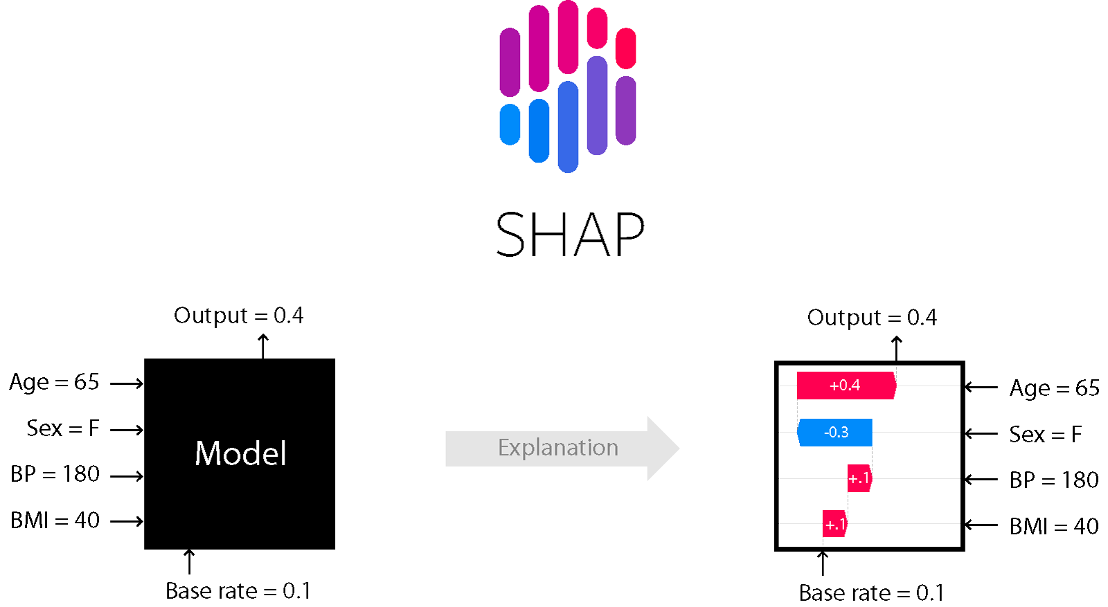
Ensemble Tree로 만족할 수준의 품질을 얻었지만 Black Box 모델의 특성상 예측 결과에 대한 명확한 해석이 쉽지 않았다. 하지만 SHAP(SHapley Additive exPlanation)[1]라는 Machine Learning 모델 해석 기법이 큰 도움이 되었다. 그 이론적 배경인 Shapley Value와 Addictive Feature Attribution Methods에 알아본 후 SHAP에 대해 알아보자.

Shapley Value

Shapley Value는 Game Theory의 알고리즘으로, Game에서 각각의 Player의 기여분을 계산하는 기법이다. Machine Learning 모델에서의 Feature Importance으로 예를 들자면 Game은 Instance(관측치)의 Prediction, Players는 Instance의 Features, 그리고 기여분은 Feature Importance로 생각할 수 있다.

 

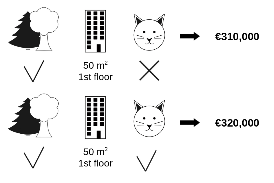
위의 그림[2]을 예로 들어보자. 해당 그림은 집 값을 예측하는 문제로 "숲세권 여부", "평수", "층", "고양이 보유여부"라는 Feature가 있다. "고양이 보유여부"의 집 값에 대한 기여분은 그 외 모든 Feature가 동일하다는 가정하에, 320,000(고양이를 키울 경우)과 310,000(고양이를 키우지 않을 경우)의 차이인 10,000이 될 것이다.

Definition

Shapley Value $\phi_i$의 계산식은 다음과 같다.

 

$$
\phi_i = \sum_{ S \subseteq F \setminus { i } } \frac{\mid S \mid! (\mid F \mid - \mid S \mid - 1)! }{\mid F \mid!} [f_{ S \cup { i } }(x_{ S \cup { i } }) - f_{S}(x_{S}) ] \\
F: the\ set\ of\ all\ features\ \\
f: prediction\ model \\
i: feature
$$

 

$\phi_i$는 기여분에 해당하는 값이다. $S \subset F$를 만족하는 모든 Feature Set $S$에 대하여 해당 Feature $i$가 있을 때와 없을 때의 Score 값의 차이 $f_{ S \cup { i } }(x_{ S \cup { i } }) - f_{S}(x_{S})$를 기여분으로 계산한다. 이 기여분을 각각의 부분 집합 $S$에 대하여, 전체 집합 $F$를 줄 세우는 경우의 수 $\mid F \mid!$ 를 $S$를 줄세우는 경우의 수 $\mid S \mid!$ 와 Feature $i$와 $S$를 제외한 나머지를 줄 세우는 경우의 수 $(\mid F \mid - \mid S \mid - 1)!$ 으로 가중평균을 한다.

Example

1. $\mid F \mid = 3, i = 1$ [3]

1, 2, 3 총 3명의 Player가 차례로 Game에 참여를 할 시, 위와 같은 순열이 가능하다. 각 경우에 대하여 Player 1 $(i=1)$의 기여분은 Player 1 참여하기 후와 전의 Value $v(\cdot)$의 차로 계산한다. 마지막으로 각 경우에 대한 개수를 가중 평균하면 Shapley Value가 계산된다.

2. Decision Tree [4]

위와 같이 학습된 Tree 모델이 있고 Feature는 $age$와 $gender$만 있다고 사정하자. $age = 14, gender = male$인 Bobby에 대하여 Feature $age$의 Shapley Value $\phi_{Age}$를 계산해보자

$\phi_{Age} : i = Age,\ F \setminus i = \{\{\}, \{x_{gender} \} \}$

$1)S =\ \{ \}$
$f_{S \cup { i }}(x_{S \cup { i }}) = \frac{(2 + 0.1)}{2} = 1.05$
$f_S(x_S) = \frac{ \frac{(2 + 0.1)}{2} + (-1) }{2} = \frac{ 1.05 - 1}{2} = 0.0025$
$\therefore \frac{\mid S \mid! (\mid F \mid - \mid S \mid - 1)! }{\mid F \mid!} [f_{ S \cup { i } }(x_{ S \cup { i } }) - f_{S}(x_{S}) ]$
$= \frac{1(2-1)!}{2!}(1.05 - 0.0025)$
$= 0.5125$

$2)\ S = \{x_{gender} \}$
$f_{S \cup { i }}(x_{S \cup { i }}) = 2$
$f_S(x_S) = \frac{ \frac{(2 + 0.1)}{2} + (-1) }{2} = \frac{ 1.05 - 1}{2} = 0.0025$
$\therefore \frac{\mid S \mid! (\mid F \mid - \mid S \mid - 1)! }{\mid F \mid!} [f_{ S \cup { i } }(x_{ S \cup { i } }) - f_{S}(x_{S}) ]$
$= \frac{1(2-1)!}{2!}(2 - 0.0025)$
$= 0.9875$

$\therefore \phi_{Age} = \sum_{ S \subseteq F \setminus { i } } \frac{\mid S \mid! (\mid F \mid - \mid S \mid - 1)! }{\mid F \mid!} [f_{ S \cup { i } }(x_{ S \cup { i } }) - f_{S}(x_{S}) ]$
$= 0.5125 + 0.9875$
$= 1.5$

Addictive Feature Attribution Methods

An explanation model that is a linear function of binary variables [5]

 

사실 Shapley Value는 Addictive Feature Attribution이라는 일반화된 Method 중 일부라 한다. Addictive Feature Attribution 은 단순한 Explanation model을 이용하여 Original Model을 해석하는 Post-hoc의 해석 기법이다. Linear function의 Weight를 이용하여 Feature의 영향력 or 중요도를 계산한다.

Definition

Addictive Feature Attribution의 정의는 다음과 같다.

$$ g(z') = \phi_{0} + \sum_{i=1}^{M}\phi_{i}z'_{i}$$

$g : explanation\ model\ (g(z') \approx f(h_x(z')))$
$f : original\ prediction\ model$
$z' \in { 0, 1 }^M : simplified\ input\ (z' \approx x')$
$h_x : mapping\ function\ (x = h_x(x'))$
$\phi_i \in \mathbb{R} : attribution\ value$
$M : the\ number\ of\ simplified\ input\ features$

여기에서 $h_x$이라는 Mapping Function에 대해 더 자세히 살펴보자. $h_x$는 Simpliified Input $x'$를 본래의 $x$로 변환해주는 임의의 Function이다. Simplified input $x'$는 $z' \approx x'$라는 가정을 통해 $x'$가 아닌 $z' \in { 0, 1 }^M$로 표현된다. Addictive Feature Attrbution은 원래의 input $x$가 아닌 Simplifiled input $z'$를 통해 $g(z') \approx f(h_x(z'))$를 만족하는 Explanation model $g$를 만드는 방법이다.

Addictive Feature Attribution의 Methods로는 LIME(Local Interpretable Model-agnostic Explanations), DeepLift, Layer-Wise Relevance Propagation, Shapley Value가 있다고 한다.

Properties

Feature Attribution은 Local Accuracy, Missingness, Consistency 이 3가지 특성 모두를 반드시 만족해야 한다고 한다.

1. Local accurracy
특정 Input $x$에 대하여 Original 모델 $f$를 Approximate 할 때, Attribution Value의 합은 $f(x)$와 같다.

$$ f(x) = g(x') = \phi_0 + \sum_{i=1}^{M} \phi_i x'_i$$

2. Missingness
Feature의 값이 0이면 Attribution Value의 값도 0이다.

$$
x'_i = 0 \Longrightarrow \phi_i = 0 \\
f_x(S \cup i) = f_x(S)
$$

3. Consistency
모델이 변경되어 어떤 Feature의 Contribution이 증가하거나 동일하다면, 그 Feature의 Attribution Value은 감소하지 않는다.

$$Let\ f_x(z') = f(h_x(z'))\ and\ z'\setminus i \ denote\ setting\ z'_i = 0. \\
f'_x(z') - f'_x(z' \setminus i) \ge f_x(z') - f_x(x' \setminus i),\ z' \in { 0, 1 }^M \\
\longrightarrow\ \phi_i(f', x) \ge \phi_i(f, x)$$

Theorem

Addictive Feature Attribution의 정의와 위 3가지 속성을 만족하는 유일한 방법은 다음 수식이다.

$$ \phi_i(f, x) = \sum_{ z' \subseteq x' } \frac{\mid z' \mid! (\mid M \mid - \mid z' \mid - 1)! }{\mid M \mid!} [f_x(z') - f_{x}(z' \setminus i) ]$$
$|z'| : the\ number\ of\ nonzero\ entries\ in\ z'$
$z' \subseteq x' : all\ z'\ vectors\ where\ the\ nonzero\ entries\ are\ a\ subset\ of\ the\ nonzero\ entries\ in\ x'$

Shapley Value는 Local Accuracy와 Consistency는 만족하지만 Missingness을 만족하지 않는다고 한다. 3가지 속성을 만족하는 방법은 해당 Theorem이 유일한 방법이라 한다.

cf) Shapley Value와의 차이점은 $i$의 기여분을 계산하는 부분이 $f_{ S \cup { i } }(x_{ S \cup { i } }) - f_{S}(x_{S})$이 아닌 $f_x(z') - f_{x}(z' \setminus i)$ 이라는 건데, Theorem은 "Missingness를 만족하기 때문에 합집합$(\cup)$의 형태가 아니어도 되는건가?" 라는 이상의 이해를 못하겠다...

 

SHAP (SHapley Additive exPlanation)

SHAP는 유일한 Additive Feature Importance Measure라 한다. Shapley values의 Conditional Expectation 버전으로 Simplified Input을 정의하기 위해 정확한 $f$ 값이 아닌 $f$의 Conditional Expectation을 계산한다

$f_x(z') = f(h_x(z'))$
$\ \ \ \ \ \ \ \ \ \ \ = f(z_S)$
$\ \ \ \ \ \ \ \ \ \ \ \approx E[f(z)\ |\ z_S]$
$h_x(z') = z_S$
$z_S : input\ has\ missing\ values\ for\ features\ not\ in\ the\ set\ S$
$S : the\ set\ of\ nonzero\ indexs\ in\ z'$

$h_x$은 Missing Value를 다루기 위해 $z'$를 $z_S$로 변환한다. $z_S$는 $S$에 존재하는 Feature의 값은 그대로 갖고 있고, 존재하지 않는 Feature는 Missing value로 처리한다. 그다음, 값이 있는 Feature에 대하여 $f$의 Conditional Expectation 값인 $E[f(z)\ |\ z_S]$을 계산한다. ($E[f(z)\ |\ z_S]$의 계산은 모델 $f$의 알고리즘마다 달라진다.)

논문의 저자가 고안한 방법의 종류로는 Tree SHAP, Kernel SHAP(Linear LIME+Shapley values), Deep SHAP(DeepLIFT+Shapley values) 등이 있다. 이 중에서도 Tree Ensemble Model에 대해 적용 가능한 Tree SHAP를 자세히 알아보자.

Tree SHAP [6]

Tree Ensemble Model의 Feature Importance를 측정하는 기존의 방법(ex. Gini, Split Count 등)들은 모델(or 개별 Tree)마다 일관되지 않은(Inconsitency) 한계점이 있다고 한다.

위 그림의 예제를 확인해보자. Tree Model인 A와 B의 Feature는 $Fever와$ $Cough$로 동일하지만 Split 순서가 다르다. Split Count 방법을 확인해보자. Model A에선 $Cough$가 2번, $Fever$가 1번 선택되어 $Cough$가 더 중요하다. 하지만 Model B에선 반대로 $Cough$가 1번, $Fever$가 2번 선택되어 $Fever$가 더 중요하다. 이 같은 현상은 Split 순서로부터 발생한다. 같은 데이터로부터 학습이 된 모델인데 모델마다 Featur Importance가 다르다면 이는 신뢰할 수 없는 값일 것이다. 하지만 SHAP는 Split 순서와 무관하게 일관된 Feature Importance를 계산할 수 있다.

저자는 Ensemble Tree 모델에 대하여 SHAP를 적용한 Tree SHAP를 제안하였다. 논문에서는 $E[f(x)\ |\ x_S]$의 계산을 Exponential time인 $O(TL2^M)$에서 Polynomial time인 $O(TLD^2)$으로 줄였다고 한다.$(T: the\ number\ of\ trees, L: maximum\ number\ of\ leaves, M: the\ number\ of\ features, D: depth\ of\ tree)$

복잡도가 Exponential time인 간단한 알고리즘의 $E[f(x)\ |\ x_S]$ 계산을 살펴보자.

$v: a\ vector\ of\ node\ values(scores))$
$a: left\ node\ indexes\ for\ each\ internal\ node$
$b: right\ node\ indexes\ for\ each\ internal\ node$
$t: thresholds\ for\ each\ internal\ node$
$d: a\ vector\ of\ indexes\ of\ the\ features\ used\ for\ splitting\ in\ internal\ nodes$
$r: the\ cover\ of\ each\ node\ (how\ many\ data\ samples\ fall\ in\ that\ sub-tree)$
$w: proportion\ of\ the\ training\ samples\ matching\ the\ conditioning\ set\ S\ fall\ into\ each\ leaf$

Input $s$와 Feature Set $S$와 한 Tree 모델 $tree = {v,a,b,t,r,d}$이 주어졌을 때, $E[f(x)\ |\ x_S]$을 계산한다. $E[f(x)\ |\ x_S]$은 $x_S$가 속하는 Leaf node의 score값과 해당 node에 속하는 Training 데이터의 비중을 곱하여 계산된다. 그 후 Ensemble 모델 Score를 계산할 때와 마찬가지로, 각 Tree의 $E[f(x)\ |\ x_S]$을 합하여 Ensemble 모델에 대한 최종 $E[f(x)\ |\ x_S]$를 계산한다.

결론 및 잡념

Shapley Value부터 시작하여 일반화된 방법인 Addictive Feature Attribution을 알아보았다. 그리고 Shapley Value의 한계점을 보완한 SHAP와 Ensemble Tree에 적용할 수 있는 Tree SHAP까지 정리해보았다.

 

개인적으로는 단순하지만 해석이 가능한 모델(ex. Regression)과 복잡하지만 해석이 불가능하는 모델(ex. Neural Network)의 중간인 Ensemble Tree를 선호하는 편이다. 하지만 모델을 설명할 때, 기존의 Feature Imporance 방법으로는 Feature '값'에 따라 y가 어떻게 변화하는지를 설명할 수 없었는데 SHAP로 인해 이제는 가능해졌다. 하지만 너무나 많은 것을 바란 것인지, Feature와 y의 인과관계를 설명하는 것은 불가능했다.'현상'을 파악을 할 순 있었지만 '왜' 그 현상이 발생하는지 까지는 알 수 없었던 것이다.

 

Feature Importance를 제대로 아는 것이 가능해진 것만으로도 너무 감사한 일이지만, 인과관계를 알기 위해서는 Causality 쪽도 공부를 해야 하는 신나는(?) 생각이 들었다.

 

Reference

[1] https://github.com/slundberg/shap
[2] Interpretable machine learning (2019)
[3] Coursera, Game Theory, 7-3 The Shapley Value
[4] https://medium.com/@gabrieltseng/interpreting-complex-models-with-shap-values-1c187db6ec83
[5] A Unified Approach to Interpreting Model Predictions (2017)
[6] Consistent Individualized Feature Attribution for Tree Ensembles (2019)